How To Use Excel's VLOOKUP to Quickly Update Product Data
It happens all the time. You get a CSV file full of products with new pricing and you’re tasked with updating the products on the website with this new data. I think we can all agree that updating product data can be a huge pain in the butt and a major time suck—especially if you’re doing it one-by-one. Well, I’m here to let you in on a little Excel secret called a VLOOKUP that’s going to make your life a whole lot easier. It sounds complicated but don’t worry, I’ll walk you through step-by-step how to perform a VLOOKUP in Excel. You’ll thank me later.
First Things First—Organize The Data
Before we get started, you’re going to need a CSV product export from your website’s database of all your current products that need updating. Most eCommerce platforms have this functionality built-in or have an add-on/extension that will allow for it. You also need the updated product data CSV (xls file will also work fine). Or, if you’d like to follow along using our example files you can download our two sample files below:
Download “outdated.csv” Download “updated.csv”
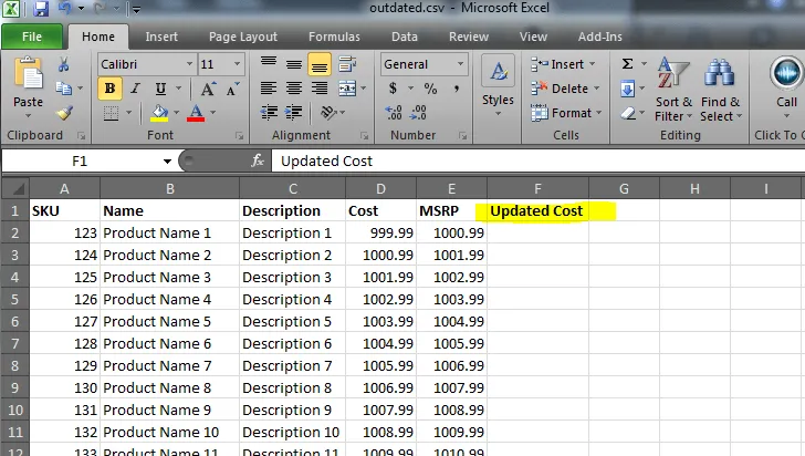
Step 1: Create a New Column
In your product database export or the “outdated.csv” in our sample files, create a new column. We’re going to be updating the cost in our example so we’ll name this column “Updated Cost”.
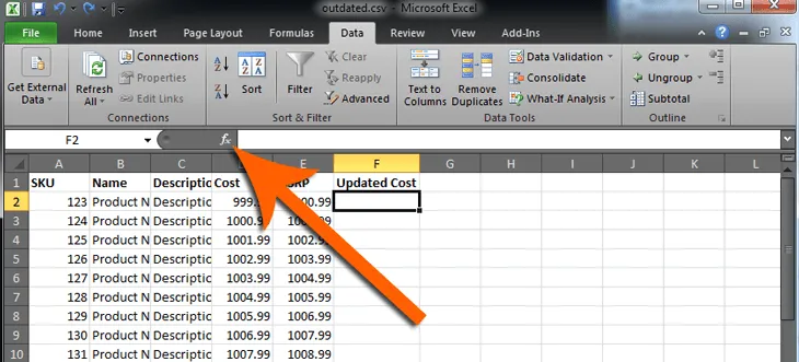
Step 2: Perform The VLOOKUP
Under the title of the new column, select the cell, click on “Insert Function” and choose VLOOKUP (the search box is your friend).
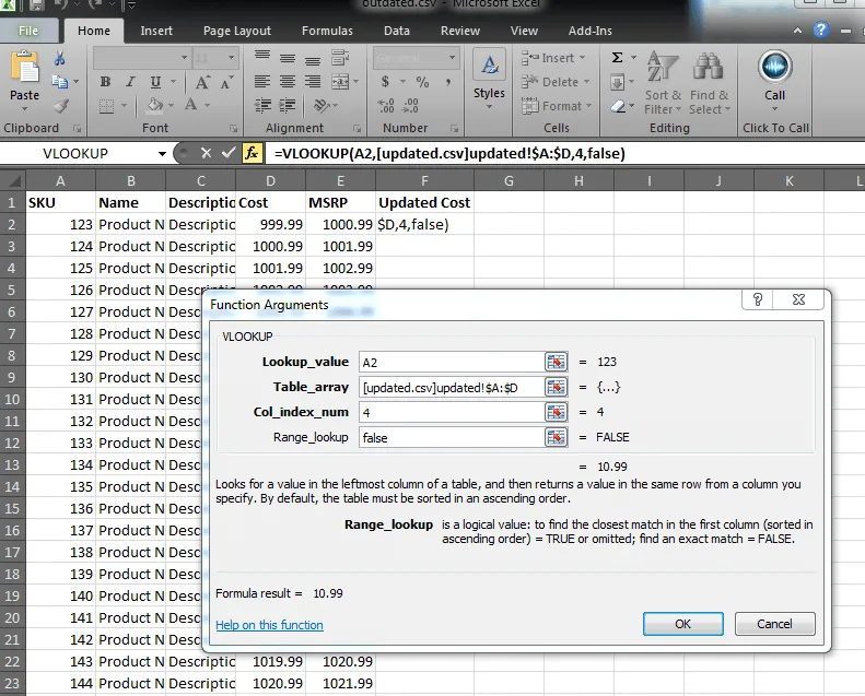
You should now see a window called “Function Arguments” that has a few empty fields. The first field titled “Lookup_value” is going to be the common attribute that is shared between the old data and the new data. In our example, we’ll use the SKU, cell A2. Got it? Good.
Select the next field titled “Table_array” and now go to the updated product data sheet “updated.csv” and select the entire column range starting from the common attribute, the SKU column, and ending with the column with the new data, the Cost column.
PROTIP: both CSV files need to be opened in the same workbook. Otherwise, you will not be able to select the “Table_array” in the other file.
Phew! If you made it this far you should start singing “she’ll be comin’ round the mountain” because we’re almost there… yeah baby!
The next field “Col_index_num” is the column data that you want to return. In other words, the column with the updated data. To find this simply count the number of columns there are from the common attribute (SKU column A) and the column with the new data (Cost column D). In our example, this number is 4.
The last field “Range_lookup” is there to specify whether you want the closest match (TRUE) or an exact match (FALSE). We’ll want to use the value FALSE.
If you followed the instructions in the sample files, your function arguments should now look like this:
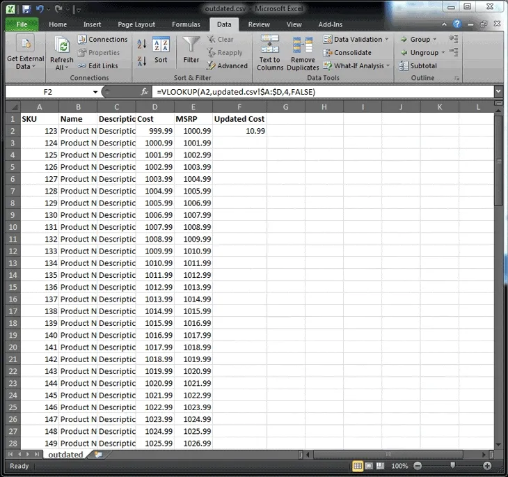
Step 3: Check The Data
Hit OK in the “Function Arguments” window and it should return the updated cost. This is where the real magic happens. Double click (or drag) the black square in the corner of the cell and the rest of the costs will populate automatically. Yes, that just happened. Yes, I just saved you hours worth of work. You’re welcome and I told you so.

At this point, you can move the updated cost into the existing cost column, save and import this sheet back into the product database.